Wave Equation

\[\frac{\partial^2 y}{\partial^2 t} = \frac{T}{\mu} \frac{\partial^2 y}{\partial^2 x}\]

Import required libraries

import matplotlib.pyplot as plt
from matplotlib.animation import FuncAnimation
import numpy as np
from IPython.display import HTML

Set up the values for the wave equation

L = 2*np.pi # Length of the string
Nx = 100 # Number of spatial points
Nt = 100 # Number of time steps
dx = L/(Nx-1) # Spatial step size
v = 5 # Wave speed
dt = np.sqrt(1)*dx/v # Time step size

print(f"dt: {dt}s")
# Initialize the spring
x = np.linspace(0, L, Nx)
y = np.zeros(Nx)
y_old = np.zeros(Nx)

# initial disturbance
y_old = np.sin(x)
# Apply fixed boundary conditions
y_old[0] = y_old[Nx-1] =  0
y[0] = y[Nx-1] =  0

#  make sure the C calculated comes out to 1
C = (v*dt/dx)**2
print(C)

dt: 0.012693303650867852s
1.0

The partial differential equation we are solving is \[ \frac{\partial^2 y}{\partial^2 t} = \frac{T}{\mu} \frac{\partial^2 y}{\partial^2 x} \] Then to solve the differential equation we can use the formula \[ y_{i+1,j}= 2y_{i,j} -y_{i-1,j} + C(y_{i,j+1} - 2y_{i,j} + y_{i,j-j}) \] where the i index represents time and the j index represents position. C is defined by \[ C=(T/\mu)(\Delta t)^2/(\Delta x)^2 \] for the first timestep, we dont have a previous time, so instead we use our initial velocity condition \(\frac{\partial y}{\partial t} = 0\) at \(t=0\) which in turn we can use the forward difference formula and the previous formula for the differential equation to gain a new formula \[ y_{i,j}= y_{i-1,j} + \frac{1}{2}C(y_{i-1,j+1} - 2y_{i-1,j} + y_{i-1,j+1j}) \] One important thing to note is that for the numerical approximation to be stable, \(C<=1\) where the theoretical solution is when equivalence holds

# compute initial timestep assuming initial velocity is 0
y[1:-1] = y_old[1:-1] + 0.5 * C * (y_old[2:] - 2 * y_old[1:-1] + y_old[:-2])
def update_string(y_old, y):
  y_new = np.zeros(Nx)
  # Use np slices to compute everything in parallel, 
  y_new[1:-1] = 2*y[1:-1] - y_old[1:-1] + C*(y[2:] - 2*y[1:-1] + y[:-2])
  # Update arrays for next iteration
  y_old[:] = y[:]
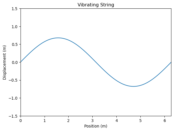
  y[:] = y_new[:]

Finally we can plot the data and also view it as an animation

# Set up the plot
fig, ax = plt.subplots()
line, = ax.plot(x, y)
ax.set_ylim(-1.5, 1.5)
ax.set_xlim(0, L)
ax.set_title('Vibrating String')
ax.set_xlabel('Position (m)')
ax.set_ylabel('Displacement (m)')
# Animation function
skip = 2
def animate(frame):
    global y_old, y, y_new, skip
    for _ in range(skip):
      update_string(y_old, y)
    line.set_ydata(y)
    return line,
# Create animation
ani = FuncAnimation(fig, animate, frames=Nt, blit=True, interval=dt*1000*skip)
ani.save('../../videos/standing_wave.mp4', writer='ffmpeg', fps=1/(dt*skip))
HTML(ani.to_jshtml())

Once Loop Reflect