Poisson’s Equation (Voltage)

\[\nabla V = -\frac{1}{\epsilon_0}\rho\]

Import required libraries

import matplotlib.pyplot as plt
from matplotlib.animation import FuncAnimation
import numpy as np
from IPython.display import HTML

Set up the data required

size = 50
voltages = np.zeros((size, size))
V0 = 50
cond = -0.5
voltages[10, 10] = V0

The partial differential equation we are solving is \[ \nabla V = -\frac{1}{\epsilon_0}\rho \]

the right hand side is cond. Then we can solve this with the boundaries of a 50x50 having a voltage of 0. To solve this we can use the following formula for \(u_{i,j}\) \[ u_{i,j} = \frac{1}{4}(u_{i,j+1}+u_{i+1,j}+u_{i,j-1}+u_{i-1,j}-cond) \]

for _ in range(500):
    for i in range(size):
        for j in range(size):
            u1 = voltages[i, j + 1] if j + 1 < size else 0
            u2 = voltages[i, j - 1] if j - 1 > -1 else 0
            u3 = voltages[i + 1, j] if i + 1 < size else 0
            u4 = voltages[i - 1, j] if i - 1 > -1 else 0
            voltages[i, j] = (u1 + u2 + u3 + u4 - cond) / 4

Then we get the gradient of this to find the electric field

pos = np.array(range(size))

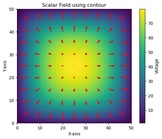
dy, dx = np.gradient(-voltages, pos, pos)

Then we graph it

skip = 5  # Number of points to skip
plt.figure()
plt.imshow(
    np.abs(voltages),
    extent=(0, size, 0, size),
    origin="lower",
    cmap="viridis",
)
plt.colorbar(label="Voltage")
plt.quiver(
    pos[::skip],
    pos[::skip],
    dx[::skip, ::skip],
    dy[::skip, ::skip],
    color="r",
    headlength=3,
)
plt.title("Scalar Field using contour")
plt.xlabel("X-axis")
plt.ylabel("Y-axis")

plt.show()