Schrödinger’s Equation

\[-\frac{\hbar}{2m}\nabla^2 \psi(x) + V(x) \psi(x) = E \psi(x)\]

Start with imports and setup

import scipy.sparse as sparse
from skimage import measure
import matplotlib.pyplot as plt
from mpl_toolkits.mplot3d import Axes3D
import plotly.graph_objects as go
import numpy as np
import torch
import time
from datetime import timedelta
from IPython.display import Image
device = torch.device('cuda' if torch.cuda.is_available() else 'cpu')

Theory

Schrödinger’s Equation is the equation governing motion at the quantum scale. We have a wavefunction \(\psi(x)\) which satisfies the following differential equation \[ -\frac{\hbar}{2m}\nabla^2 \psi(x) + V(x) \psi(x) = E \psi(x) \]

We can then see that this differential equation actually forms an eigenvector problem or more specifically, \[ \hat{H} \ket{\psi} = (\hat{T} + \hat{V})\ket{\psi} = E \ket{\psi} \]

we can then find the central difference of \(\frac{d^2 \psi}{dx^2}\), being \[ \frac{d^2 \psi}{dx^2} = \frac{\psi_{x-1}-2\psi_x+\psi_{x+1}}{(\Delta x)^2} \]

The next step is to recognize our boundary conditions, which for us is \(\psi(0)=\psi(L)=0\). Then we can represent \(\hat{H}\) as a discrete matrix instead of an arbitrary linear operator, given our finite difference as \[ \hat{H} = -\frac{\hbar}{2m(\Delta x)^2}D+V \] Where \(D\) and \(V\) are matrices representing the Laplacian and Potential, represented as such \[ D = \begin{pmatrix} -2 & 1 & 0 \\ 1 & -2 & 1 \\ 0 & 1 & -2 \\ \end{pmatrix}, V= \begin{pmatrix} V_1 & 0 & 0 \\ 0 & V_2 & 0 \\ 0 & 0 & V_3 \\ \end{pmatrix} \] Given we have three datapoints each diagonal entry in \(V\) is the voltage at that given position. These matrices are then “extended” to fit within the number of datapoints we have, making sure to keep the matrix hemertian.

However what if we want to extend this to higher dimensions. Then we need to take what is known as a kroneker sum of the matrix \(D\) and use it in its place. It is defined as so \[ D \oplus D = D \otimes I + I \otimes D \] where \(\otimes\) is the kroneker product and is defined as \[ D \otimes I = \begin{pmatrix} D & 0 & 0\\ 0 & D & 0\\ 0 & 0 & D\\ \end{pmatrix} \] then for 2 dimensions we just use one kroneker sum and for 3 dimensions we can use 3 as so \[ D \oplus D \oplus D \] which happens to work out. Then we can flatten our grid of sample points and make it a simple n dimensional vector our final equation then becomes \[ \left[\frac{\hbar}{2m}(D\oplus D\oplus D)+V\right]\vec{\psi} = E \vec{\psi} \] which we can simplify using natural units, setting \(\hbar = 1\) and as well making the entries in \(V\) return \(m\delta^2V(x,y,z)\) as well as the energy eigenvalues being now \(m\delta^2E\), where \(\delta\) is a generalized finite differential for all directions in space. This becomes the following equation then \[ \left[\frac{1}{2}(D\oplus D\oplus D)+V\right]\vec{\psi} = m\delta^2E \vec{\psi} \] Noting that the matrix \(V\) itself is returning a different value now of \(m\delta^2V(x)\)

Calculations

With this we can finally start on the calculations. Start by defining a Potential (Noting this is really potenetial energy and not electric potential). The potential is then the potential energy of an electron in an atom of hydrogen which is \[ V(r) = -\frac{e^2}{4 \pi \epsilon_0 r} = -\frac{1}{ma_0 r},\, a_0 = \frac{4\pi\epsilon_0\hbar^2}{e^2m}\approx 5.29 \times 10^-11m \] This allows us to define the radius in terms of the bohr radius \(a_0\). We can then rearange the equation to solve for \(m\delta^2V(x)\) and write our function as \[ m\delta^2V(x)= -\frac{\delta^2}{a_0 r} = -\frac{(\delta/a_0)^2}{(r/a_0)} \] Changing the units to a_0 by dividing by \(a_0/a_0\)

Start by defining values for our grid and delta

N = 120
# Note that both the coordinates and delta are measured in units of a_0
X,Y,Z = np.mgrid[-25:25:N*1j,-25:25:N*1j,-25:25:N*1j] # create a grid from -25 to 25 a_0
delta = np.diff(X[:,0,0])[0] # get the step size

Now we write a function to get the potential as follows

def get_potential(x,y,z):
  # since the units are in a_0 we can treat the a_0 in the equation defined above as 1
  # As well we add 1e-10 to the value of r to avoid any infinities at r=0
  return -delta**2/np.sqrt(x**2+y**2+z**2 + 1e-10)

V0 = get_potential(X,Y,Z) # This creates a 3d grid of potentials
V0.shape # shape should be n*n*n we really want this to be a diagonal matrix in M_{n^3}(R)

(120, 120, 120)

We want to get our proper \(V\) matrix which we can do along with our \(D\) matrix

diag = np.ones([N]) # create a vector of ones in R^n
diags = np.array([diag, -2*diag, diag]) # create a n*3 matrix representing the diagonals in D
D = sparse.spdiags(diags, np.array([-1,0,1]), N, N) # Create D from the diags
T = -1/2 * sparse.kronsum(sparse.kronsum(D,D), D) # Create T from D
V = sparse.diags(V0.reshape(N**3), (0)) # Create a sparse matrix from V0
H = T+V # Finally create the hamiltonian matrix
H.shape # Print out the shape of H which should be (N^3,N^3)

(1728000, 1728000)

Convert H so that it is on the gpu. This makes finding the eigenvalues easier

H = H.tocoo()
H = torch.sparse_coo_tensor(indices=torch.tensor([H.row, H.col]), values=torch.tensor(H.data), size=H.shape).to(device)

/tmp/ipykernel_248606/2973072149.py:2: UserWarning:

Creating a tensor from a list of numpy.ndarrays is extremely slow. Please consider converting the list to a single numpy.ndarray with numpy.array() before converting to a tensor. (Triggered internally at /build/python-pytorch/src/pytorch/torch/csrc/utils/tensor_new.cpp:254.)

Finally we can compute the eigenvalues/eigenvectors as follows

num_states = 20 # number of states to calculate
start = time.perf_counter()
eigenvalues, eigenvectors = torch.lobpcg(H, k=num_states, largest=False)
end = time.perf_counter()
elapsed = timedelta(seconds = end-start)
print("Time to calculate:", elapsed)

Time to calculate: 0:43:18.962407

Here is a function to get a an eigenvector given an energy level

def get_e(n):
    return eigenvectors.T[n].reshape((N,N,N)).cpu().numpy()

We can compute an object given a certain energy level and plot it

eigenstate = 6 # Eigenstate to display
verts, faces, _, _ = measure.marching_cubes(get_e(eigenstate)**2, 1e-6, spacing=(0.1, 0.1, 0.1))
intensity = np.linalg.norm(verts, axis=1)

fig = go.Figure(data=[go.Mesh3d(x=verts[:, 0], y=verts[:, 1], z=verts[:, 2], 
                                i=faces[:, 0], j=faces[:, 1], k=faces[:, 2],
                                intensity=intensity,
                                colorscale='Agsunset',
                                opacity=0.5)])

fig = fig.update_layout(scene=dict(xaxis=dict(visible=False),
                              yaxis=dict(visible=False),
                              zaxis=dict(visible=False),
                              bgcolor='rgb(0, 0, 0)'),
                  margin=dict(l=0, r=0, b=0, t=0))

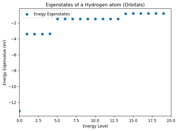
fig.show()

plot the eigenvalues by first converting the units to joules

hbar = 1.055e-34
a0 = 5.29e-11
m = 9.11e-31 # Mass of an electron
J_to_eV = 6.242e18 # convert from Joules to eV
conversion = hbar**2 / m / delta**2 / a0**2 * J_to_eV 
converted_eigenvalues = eigenvalues.cpu() * conversion

plt.figure()
plt.scatter(list(range(num_states)), converted_eigenvalues, label="Enegy Eigenstates")
plt.xlim(0,20)
plt.title("Eigenstates of a Hydrogen atom (Orbitals)")
plt.xlabel("Energy Level")
plt.ylabel("Energy Eigenvalue (eV)")
plt.legend()
plt.show()