Geodesics

\[\frac{d v^\mu}{d \tau} + \Gamma^\mu_{\alpha \beta} v^\alpha v^\beta = 0\]

The geodesic equation is a first order ode for the tangent vector to a geodesic. It can be written as

\[ \frac{d v^\mu}{d \tau} + \Gamma^\mu_{\alpha \beta} v^\alpha v^\beta = 0 \]

And \(\Gamma^\mu_{\alpha \beta}\) is the Christoffel symbol, which can be computed from the metric \(g_{\mu \nu}\) as

\[ \Gamma^\mu_{\alpha \beta} = \frac{1}{2} g^{\mu \gamma} \left( \partial_\alpha g_{\beta \gamma} + \partial_\beta g_{\alpha \gamma} - \partial_\gamma g_{\alpha \beta} \right) \]

where \(\partial_{\alpha}\) is short for \(\frac{\partial}{\partial x^\alpha}\). Then using the metric of a sphere, we get that

\[ g_{\mu \nu} = \begin{pmatrix} R^2 & 0 \\ 0 & R^2 \sin^2 \theta \end{pmatrix} \]

Now let us compute the Christoffel symbols, through numerical code. First we import the necessary libraries, and then we define the metric and its inverse. We also define a function to compute the Christoffel symbols from the metric.

import numpy as np
def metric(theta, phi, R=1):
  theta = np.asarray(theta)
  g = np.zeros((2, 2, len(theta)))
  g[0, 0] = R**2
  g[1, 1] = R**2 * np.sin(theta)**2
  return g

def inverse_metric(theta, R=1):
  theta = np.asarray(theta)
  g_inv = np.zeros((2, 2, len(theta)))
  g_inv[0, 0] = 1 / R**2
  g_inv[1, 1] = 1 / (R**2 * np.sin(theta)**2)
  return g_inv

Now we numerically compute the christoffel symbols using the metric and its inverse:

def deriv(f, x, delta=1e-5):
  x1 = x + delta
  x2 = x - delta
  return (f(x1) - f(x2)) / (x1 - x2)

def deriv_metric(point, R, var, delta=1e-5):
  theta, phi = point
  return deriv(lambda x: metric(
    x if var == 0 else theta,
    x if var == 1 else phi, R),
    phi if var == 1 else theta, delta)


def christoffel_symbols(point, R=1):
  theta, phi = point
  theta = np.asarray(theta)
  g = metric(theta, phi, R)
  g_inv = inverse_metric(theta, R)
  Gamma = np.zeros((2,2,2, len(theta)))


  for mu in range(2):
    for alpha in range(2):
      for beta in range(2):
        for gamma in range(2):
          Gamma[mu, alpha, beta] += (g_inv[mu, gamma]/2)*(
            deriv_metric(point, R, beta)[gamma, alpha] +
            deriv_metric(point, R, alpha)[gamma, beta] -
            deriv_metric(point, R, gamma)[alpha, beta])

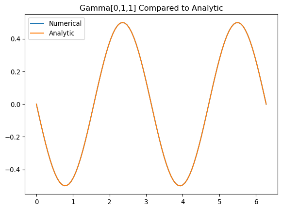
  return Gamma

To check if the numerical calculation is valid, we can plot the individual components over theta.

import matplotlib.pyplot as plt
thetas = np.linspace(0, 2*np.pi, 100)
points = np.array([
    thetas,
    np.zeros_like(thetas)
  ])

Gammas = christoffel_symbols(points)

plt.plot()
plt.title("Gamma[0,1,1] Compared to Analytic")
plt.plot(thetas, Gammas[0,1,1], label=f"Numerical")
plt.plot(thetas, -np.sin(thetas)*np.cos(thetas), label=f"Analytic")
plt.legend()
plt.show()

/tmp/ipykernel_17803/1483375053.py:13: RuntimeWarning:

divide by zero encountered in divide

/tmp/ipykernel_17803/1989934059.py:26: RuntimeWarning:

invalid value encountered in multiply

plt.plot()
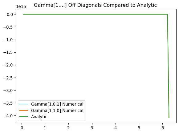
plt.title("Gamma[1,...] Off Diagonals Compared to Analytic ")
plt.plot(thetas, Gammas[1,0,1], label=f"Gamma[1,0,1] Numerical")
plt.plot(thetas, Gammas[1,1,0], label=f"Gamma[1,1,0] Numerical")
plt.plot(thetas, 1/np.tan(thetas), label=f"Analytic")
plt.legend()
plt.show()

/tmp/ipykernel_17803/3004824766.py:5: RuntimeWarning:

divide by zero encountered in divide

plt.plot()
plt.title("Zeroes of Gamma")
plt.plot(thetas, Gammas[0,0,0], label=f"Gamma[0,0,0] Numerical")
plt.plot(thetas, Gammas[0,0,1], label=f"Gamma[0,0,1] Numerical")
plt.plot(thetas, Gammas[0,1,0], label=f"Gamma[0,1,0] Numerical")

plt.plot(thetas, Gammas[1,0,0], label=f"Gamma[1,0,0] Numerical")
plt.plot(thetas, Gammas[1,1,1], label=f"Gamma[1,1,1] Numerical")
plt.legend()
plt.show()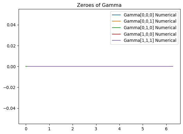

Since all of these are acurate to the analytic Christoffel Symbols we can go on to the geodessic equation

Geodessic Equation

To solve the Geodessic equation, we can solve the resulting system of ODEs Numerically

from scipy.integrate import solve_ivp
def geodesic_equation(tau, state, R=1):
  theta, phi, v_theta, v_phi = state
  point = np.array([[theta], [phi]])
  Gamma = christoffel_symbols(point, R)
  d_v_theta_dtau = -Gamma[0,0,0]*v_theta**2 - 2*Gamma[0,0,1]*v_theta*v_phi - Gamma[0,1,1]*v_phi**2
  d_v_phi_dtau = -Gamma[1,0,0]*v_theta**2 - 2*Gamma[1,0,1]*v_theta*v_phi - Gamma[1,1,1]*v_phi**2
  return [v_theta, v_phi, d_v_theta_dtau[0], d_v_phi_dtau[0]]

initial_state = [np.pi/4, 0, 0, 1]  # Initial conditions: theta, phi, v_theta, v_phi
time_span = (0, 10)  # Time span for integration
solution = solve_ivp(geodesic_equation, time_span, initial_state, t_eval=np.linspace(time_span[0], time_span[1], 100))

plt.figure()
plt.plot(solution.y[0], solution.y[1])
plt.title("Geodesic on a Sphere")
plt.xlabel("Theta")
plt.ylabel("Phi")
plt.show()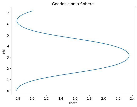

Now lets plot it on a sphere interactively using plotly

import plotly.graph_objects as go
R = 1
x = R*(np.sin(solution.y[0]) * np.cos(solution.y[1]))
y = R*(np.sin(solution.y[0]) * np.sin(solution.y[1]))
z = R*(np.cos(solution.y[0]))

#thetas = np.linspace(0, np.pi, 50)
#phis = np.linspace(0, 2*np.pi, 50)
d = np.pi/32
thetas, phis= np.mgrid[0:np.pi+d:d, 0:2*np.pi+d:d]
circle_x = (R * np.cos(phis) * np.sin(thetas)).ravel()
circle_y = (R * np.sin(phis) * np.sin(thetas)).ravel()
circle_z = (R * np.cos(thetas)).ravel()


fig = go.Figure(data=[
  go.Mesh3d(x=circle_x, y=circle_y, z=circle_z, opacity=1, color='lightblue', alphahull=0),
  go.Scatter3d(x=x, y=y, z=z, mode='lines', line=dict(color='red', width=5))
])

fig.update_layout(title='Geodesic on a Sphere', scene=dict(
    xaxis_title='X',
    yaxis_title='Y',
    zaxis_title='Z'
))
fig.show()