RLC Circuit

\[\frac{1}{s^2LC + sRC + 1}\]

Start with imports

import numpy as np
from scipy import signal
import matplotlib.pyplot as plt

An RLC circuit can be described with the language of Laplace Transforms and Transfer Functions. This ammounts to the Phasor representation of circuits.

Take a simple RLC circuit with the impedance

\[ Z(s) = R + sL + \frac{1}{sC} \]

The transfer function of this circuit is

\[ H(s) = \frac{V_{out}}{V_{in}} \]

Our output voltage is the capacitor, which is

\[ V_c = V_{in} \times \frac{Z_c}{Z(s)} = V_{in} \frac{\frac{1}{sC}}{R + sL + \frac{1}{sC}} = V_{in} \frac{1}{s^2LC + sRC + 1} \]

Then our final transfer function is

\[ H(s) = \frac{V_{in} \frac{1}{s^2LC + sRC + 1}}{V_{in}} = \frac{1}{s^2LC + sRC + 1} \]

We can set our circuit values to the following

R = 100.0          # ohms
L = 100e-6         # henries
C = 10e-6          # farads

Then define our system like so

num = [1.0]
den = [L*C, R*C, 1.0] # in descending order of degree

system = signal.TransferFunction(num, den)

The resonant frequency of an RLC circuit is defined as

\[ f_{res} = \frac{1}{2\pi \sqrt{LC}} \]

In the s-domain, the imaginary component represents angular frequency which allows us to define the resonant frequency at the poles of this function at some given \(\omega\).

We can start by writing he denominator in standard form

\[ s^2 + \frac{R}{L} s + \frac{1}{LC} \]

The resonant frequency makes the denominator 0 (and therefore makes our transfer function blow out to infinity). This means we want to find roots of this function such that they are solely imaginary. The general roots are given by the quadratic formula

\[ s = \frac{-R/L \pm \sqrt{R^2/L^2 - 4/LC}}{2} \]

if this were to be purely imaginary, that means that \(R = 0\) (this implies resistance leads to damping and we can never remove resistance physically, which is why we dont blow out to infinity) Then this implies that

\[ s = \pm \frac{i}{\sqrt{LC}} \]

We then define the resonant frequency at \(s = i \omega\), ignoring the sign as negative frequency doesnt change the inherent meaning of the frequency, to get.

\[ \omega = \frac{1}{\sqrt{LC}} \]

Which obviously implies the formula we already found. To actually simulate the system, we can supply a signal to it like so

freq = 440
omega = freq*2*np.pi
t = np.linspace(0,4/freq,100)
V_in = signal.square(omega*t) 
tout, y, x = signal.lsim(system, V_in, t)

Then plot the system as the following

plt.figure()
plt.title("Voltage Drop of an RLC Circuit")
plt.xlabel("Time (s)")
plt.ylabel("Voltage (V)")
plt.plot(t, V_in, label="Input")
plt.plot(t, y, label="Output")
plt.legend(loc="lower right")
plt.show()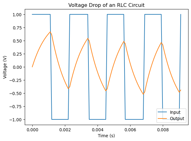

From this you can see we get a realistic simulation of the voltage in an RLC circuit. One further test would be to check if this circuit produces a similar output experimentally, which is something I might consider in the future given the oportunity.